A decades of metagenomics approach based studies, a text mining overview
The microbiota is the sum of microbial element of a given ecosystem which can be ocean, soils or human body site like oral and gut. In the 90’s, scientist studied microbiota using classical microbiology culture-dependent approach. However, the majority of microbes aren’t cultivable yet and trying to understand interaction in a microbial ecosystem is clearly biased without independent culture approach.
Rondon et al published in 2000 for the first time a soil study using the metagenomic approach. Basically, it consist to study all the DNA extracted from an environmental sample. As a result, whereas the number of microbiota study continued to increase, the number of paper using metagenomic took off. The metagenomic approach is the “association” of environmental ecology and genomic.
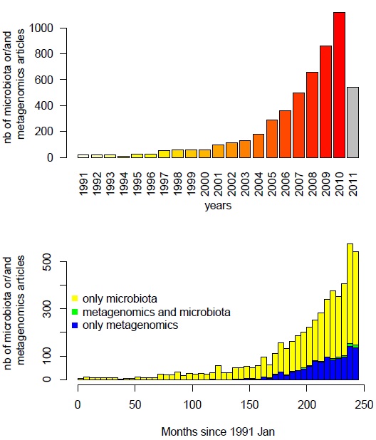
I always got the feeling from my lecture than this full association was not done between ecologist and genomic people. To test this association, I extracted the 10/04/2011 from the pubmed database all articles with this query : give me article where you find in title or in the abstract the keyword “metagenomic” or “microbiota” since 1991. With this query, I obtained 5193 articles.

On the top panel it’s clear that the number of paper on this domain increase exponentially since the 90’s and we can bet that the number of article in 2011 will be higher than 2010. Surprisingly, on the bottom panel, whereas “metagenomic” and “microbiota” keywords are more and more used (yellow and blue bars), very few articles used both (green bars) in the same time in their title or abstract.
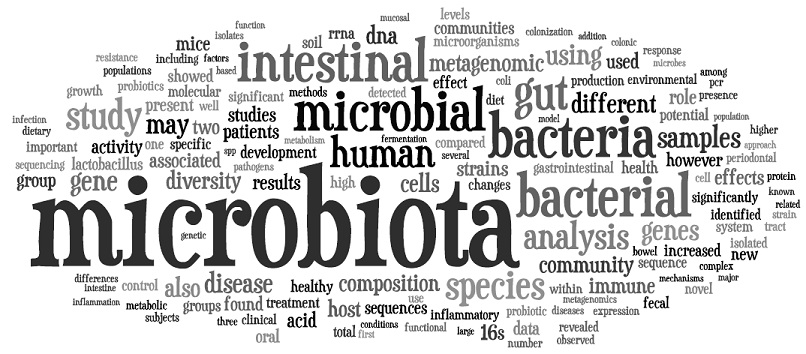
Why so few overlap between metagenomic and microbiota paper ? Maybe this two keywords are too restrictive too explain how metagenomic impacted microbial ecology… so in the way to explore further I selected all keyword appeared at least 100 times from the whole title and abstract dataset (5193 article). I removed usual common english term like “was”, “it”, “has”, “the” and I obtained finally 1023 keywords. Despite the fact that “microbiota” is a most used keyword, there is some variation like “microbial”, “bacterial”, “bacteria”. By the way, other keyword pop up like “disease”, “intestinal”, “gut” or “gene” … maybe they will help us to understand this non-association between microbiota and metagenomic.

Then, I searched the presence or absence of this keyword in article titles and abstracts. From this presence/absence matrix, an multiple correspondance analysis was done and from this a between class analysis was computed regrouping articles by their publication year.
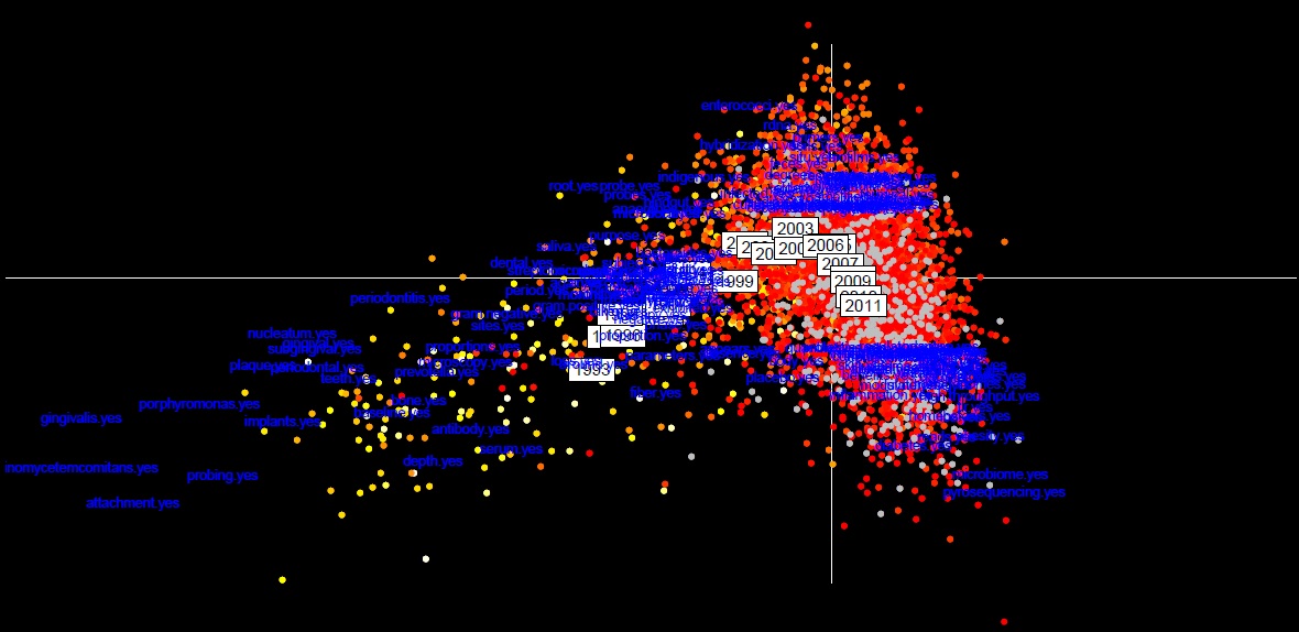
The first axis which represent the first component of the analysis represent the major message of this dataset. It’s clear that there is a gradient according the time (years). Most keyword used in the 90’s were related to the oral microbiota using observation technique like microscopy. Until 1999, the oral microbiota is less and less studied compared to others like soils, ocean and fecal microbiota and the apparition of molecular tools technique like Fluoresence Hybridization In Situ (FISH) and the utilization of nucleotide probes and primers. Then in 2000, there is more and more metagenomic studies using high throughput technology like pyrosequencing. However, until 2010 (and also in 2011) there is a clear focus only on human microbiota in relation with clinical keyword like obesity and diabetes which are the clear trends nowadays. Interestingly concerning bacterial genera, Prevotella and Porphyromonas were broadly studied in the 90’s isolated from the oral microbiota but in 2010, it’s clear that Bacteroides bacteria are now mainly studied isolated from fecal microbiota.
On the second axis which represent the second message, we can see that on the same time, ecologist people continue to analyzed their preferred ecosystem with old fashion technique whereas genomic people focus mainly on human for clinical purpose.
Genomic people use microbial sequenced genome to bin metagenomic dataset, we can question the fact that microbial strains were chosen based on scientific interested… i.e. Prevotella for oral microbiota and Bacteroides for fecal microbiota may then cause a bias in the analysis.
####Methods
Here is the boolean query in pubmed :
(metagenomic*[Title/Abstract] OR microbiota[Title/Abstract])
AND "1991"[Publication Date] : "2011"[Publication Date]
Then, the xml result file was downloaded and parsed by Microsoft Excel. The xml file and a filtered tabular file are available here.
here is the R code:
	#load ade4 library
	require(ade4)

	#read table
	read.table("metagenomics.microbiota.1991.2011.tab.txt", sep="\t", header=T) -> meta
	as.character(meta$PMID)-> meta$PMID
	as.factor(meta$Year) -> meta$Year
	as.factor(meta$Month) -> meta$Month

	#Histogram
	par(mfrow=c(2,1), mar=c(5,5,1,1))
	barplot(table(meta$Year), las=2, col=c(rev(heat.colors(20)), "grey"), ylab="nb of microbiota or/and \n metagenomics articles", xlab="years")
	hist(meta$Month2, breaks=42, main="", xlab="Months since 1991 Jan", ylab="nb of microbiota or/and \n metagenomics articles", col="yellow")
	hist(meta$Month2[which(meta$metagenomic=="yes" | meta$metagenomics=="yes")],col="green",breaks=42, add=T)
	hist(meta$Month2[which(meta$microbiota=="no" & meta$metagenomic=="yes" | meta$metagenomics=="yes")],col="blue",breaks=21, add=T)
	legend("left", c("only microbiota","metagenomics and microbiota", "only metagenomics"), pch=15, col=c("yellow","green","blue"), bty="n")

	#between class analysis and ACM
	dudi.acm(meta[,c(7:1029)], scan=F, nf=3) -> meta.acm
	between(meta.acm, fac=factor(meta$Year), scann=F) -> meta.year.bet

 	#plot 2 first component
	par(bg="black")
	s.class(meta.year.bet$ls, fac=(meta$Year), cell=0, cstar=0, col=c(rev(heat.colors(20)), "grey"), grid=F)
	abline(h=0, col="white", lty=2)
	abline(v=0, col="white", lty=2)
	s.class(meta.year.bet$ls, fac=(meta$Year), cell=0, cstar=0, col=c(rev(heat.colors(20)), "grey"), grid=F, add.plot=T)
	s.label(meta.year.bet$li, add.plot=T)
	which(meta.year.bet$co[,1] > 0.4 | meta.year.bet$co[,1]  0.2 | meta.year.bet$co[,2]) ->  select
	text(meta.year.bet$co[select, 1:2]/2.5, label=row.names(meta.year.bet$co[select,]), cex=0.8, col="blue")
